Calculating RESP charges with pre-computed ESPs

In some cases you may already have computed grids and electrostatic potentials for a known molecule geometry, either using PsiRESP or another library. In this case, you can use a minimal installation of PsiRESP without RDKit, QCFractal, or Psi4 to calculate charges using various methods.

This tutorial presumes that you are already familiar with the basic concepts of RESP charges and using PsiRESP. If not, please see the related notebooks:

If you have not pre-computed ESPs but you still do not want to use a QCFractal, please see:

Calculating RESP charges without a server

This tutorial uses the same molecules as Calculating charges of multiple molecules with a temporary server.

Pandas is an optional library used for organising and plotting the data at the end.

[1]:

import psiresp
import qcelemental as qcel
import numpy as np
import pandas as pd

%matplotlib inline

Creating the molecules

We load in two molecules from XYZ files. For demonstration purposes, this file is from the PsiRESP testing files.

[2]:

from psiresp.tests.datafiles import (
    NME2ALA2_OPT_C1
    METHYLAMMONIUM_OPT
)

We create QCElemental molecules and then PsiRESP molecules, step-by-step. nme2ala2 will be a simple molecule with only one conformer and one orientation. methylammonium will be a slightly more complex molecule with one conformer, and two orientations per conformer, to demonstrate full capability.

Please see the documentation on Orientations for an explanation of why we use multiple orientations for a molecule, and which orientations can be specified or automatically generated.

[3]:

nme2ala2_c1 = qcel.models.Molecule.from_file(
    NME2ALA2_OPT_C1,
    dtype="xyz",
)
menh3 = qcel.models.Molecule.from_file(
    METHYLAMMONIUM_OPT,
    dtype="xyz",
    molecular_charge=1,
)

It is highly recommended to create PsiRESP molecules by adding Conformers one-by-one, as validation checks are run for each new conformer. You can add a conformer both with add_conformer if you are using a QCElemental molecule, or with add_conformer_with_coordinates if you only have coordinates. add_conformer_with_coordinates allows a units keyword for conversion.

[4]:

nme2ala2 = psiresp.Molecule(qcmol=nme2ala2_c1)
nme2ala2.add_conformer_with_coordinates(nme2ala2_c1.geometry, units="bohr")

Alternatively, if you are only using one conformer, you do not need to directly add a conformer at all.

[5]:

methylammonium = psiresp.Molecule(qcmol=menh3, charge=1)
methylammonium.generate_transformations(n_reorientations=2)
methylammonium.reorientations

# alternatively, you can specify:
# methylammonium = psiresp.Molecule(
#     qcmol=menh3,
#     reorientations=[(0, 4, 1), (1, 4, 0)],
#     charge=1,
# )

[5]:

[(0, 4, 1), (1, 4, 0)]

Adding the grid and ESP values

The grids and ESP values are properties of psiresp.Orientation objects. These can be added manually using Conformer.add_orientation_with_coordinates(), analogous to Molecule.add_conformer_with_coordinates() above. However, if we are not specifying multiple orientations, we can simply use the geometries we passed in initially. This occurs automatically when we call Molecule.generate_orientations().

[6]:

nme2ala2.generate_orientations()
methylammonium.generate_orientations()

With Orientations generated, we can add the grid and ESP directly to the Orientation.grid and Orientation.esp properties. Again, we load this from the PsiRESP test data files

[7]:

import numpy as np
from psiresp.tests.datafiles import (
    NME2ALA2_OPT_C1_GRID,
    NME2ALA2_OPT_C1_ESP,
    METHYLAMMONIUM_O1_GRID,
    METHYLAMMONIUM_O1_ESP,
    METHYLAMMONIUM_O2_GRID,
    METHYLAMMONIUM_O2_ESP,
)

nme2ala2.conformers[0].orientations[0].grid = np.loadtxt(NME2ALA2_OPT_C1_GRID)
nme2ala2.conformers[0].orientations[0].esp = np.loadtxt(NME2ALA2_OPT_C1_ESP)
methylammonium.conformers[0].orientations[0].grid = np.loadtxt(METHYLAMMONIUM_O1_GRID)
methylammonium.conformers[0].orientations[0].esp = np.loadtxt(METHYLAMMONIUM_O1_ESP)
methylammonium.conformers[0].orientations[1].grid = np.loadtxt(METHYLAMMONIUM_O2_GRID)
methylammonium.conformers[0].orientations[1].esp = np.loadtxt(METHYLAMMONIUM_O2_ESP)

Generating charge constraints

Below, we generate an inter-molecular charge constraint. Without RDKit, we need to specify the constraint with atom indices instead of SMILES or SMARTS. We are able to do this because we specified the geometry ourselves from the XYZ file, so we can use a visualisation program such as nglview or VMD to pick out the correct atoms. The below constraint sums the methyl group from methylammonium and the acetyl group from nme2ala2 to equal 0.

[8]:

constraints = psiresp.ChargeConstraintOptions()
methyl_atoms = methylammonium.get_atoms(indices=[0, 2, 3, 4])
ace_atoms = nme2ala2.get_atoms(indices=[0, 1, 2, 3, 11, 12, 13, 14])
constraint_atoms = methyl_atoms + ace_atoms
constraints.add_charge_sum_constraint(charge=0, atoms=constraint_atoms)

Running the job

As previously, we can create a typical psiresp.Job and calculate charges. Instead of calling Job.run(), we need to use Job.compute_charges – Job.run() will always try to re-compute ESPs, to ensure that they match up to the given grid.

[9]:

job = psiresp.Job(molecules=[nme2ala2, methylammonium], charge_constraints=constraints)
normal_charges = job.compute_charges()
normal_charges

[9]:

[array([-0.3479946526284455,  0.0947455215646185,  0.0947455215646185,
         0.0947455215646184,  0.7867893485647182, -0.5839738350665387,
        -0.6944927712231437,  0.3442376495266471,  0.2608201018834638,
         0.3357773566071751, -0.0806738394616683, -0.0806738394616684,
        -0.0806738394616686, -1.2940908358803895,  0.3662001565578509,
         0.3662001565578512,  0.3662001565578511,  0.6748251608445328,
        -0.5559612286597867, -0.5100631453864023,  0.3016945866012605,
        -0.1972274084181829,  0.1129480524175629,  0.1129480524175629,
         0.1129480524175629]),
 array([ 2.4385815262909025, -0.4054676074142619, -0.405467607414262 ,
        -0.4054676074142622, -0.4746498652819122,  0.0544943887160196,
         0.0989882067931542,  0.0989885657246218])]

The charges above are computed with 2-stage RESP with a hyperbolic restraint, and typical coefficients used in the restraint (restraint_slope=0.1, restraint_height_stage_1=0.0005, restraint_height_stage_2=0.001)

[10]:

job.resp_options

[10]:

RespOptions(restraint_slope=0.1, restrained_fit=True, exclude_hydrogens=True, convergence_tolerance=1e-06, max_iter=500, restraint_height_stage_1=0.0005, restraint_height_stage_2=0.001, stage_2=True)

One reason to use PsiRESP, even if you already have pre-computed geometries, grids, and electrostatic potentials, is being able to easily fit charges to different options. For example, changing the restraint slope:

[11]:

job.resp_options.restraint_slope = 1
slope_1 = job.compute_charges()
slope_1

[11]:

[array([-0.4545908255000874,  0.1207242780390815,  0.1207242780390815,
         0.1207242780390817,  0.8778592164258321, -0.6057686634879043,
        -0.8459350984200689,  0.381823108747242 ,  0.3771341049247636,
         0.3416614212413097, -0.0904680402945985, -0.0904680402945986,
        -0.0904680402945988, -1.2034314715179415,  0.3327264233352316,
         0.3327264233352314,  0.3327264233352314,  0.6979337100609917,
        -0.5734125251129846, -0.5413040869769363,  0.325712154393496 ,
        -0.267247534312278 ,  0.1335395020984744,  0.1335395020984745,
         0.1335395020984745]),
 array([ 2.4750043684883614, -0.4143512615178306, -0.4143512615178305,
        -0.4143512615178303, -0.5022427252979501,  0.0602535036503358,
         0.1050191406545201,  0.105019497058224 ])]

We might also change the restraint height:

[12]:

job.resp_options.restraint_height_stage_1 = 1
height_1 = job.compute_charges()
height_1

[12]:

[array([-0.0247748721379307,  0.052922211872479 ,  0.052922211872479 ,
         0.0529222118724789, -0.0207917828185526, -0.0977226352361417,
        -0.0078511052684009,  0.170124202725129 , -0.0121162862918905,
        -0.0390820673420221,  0.0735757457230962,  0.0735757457230962,
         0.0735757457230963, -1.205388670315887 ,  0.3207989618176216,
         0.3207989618176214,  0.3207989618176218, -0.0439126788205824,
        -0.0951905340534581, -0.0230484017145005,  0.078675143363542 ,
        -0.3664773104777325,  0.1152220800496126,  0.1152220800496127,
         0.1152220800496128]),
 array([ 0.2929154736940858,  0.1617760533253261,  0.1617760533253263,
         0.1617760533253263, -0.0130211267721713,  0.0591071102863873,
         0.0878350394224338,  0.0878353433932856])]

Or turn off charge constraints:

[13]:

job.charge_constraints.charge_sum_constraints = []
no_constraints = job.compute_charges()
no_constraints

[13]:

[array([ 0.0327256134724813,  0.0387696031046107,  0.0387696031046106,
         0.0387696031046106, -0.0275298364658156, -0.0942734144329204,
        -0.0112955162349269,  0.150869444329444 , -0.0226591029864556,
         0.3020894839251422, -0.0171308284066392, -0.0171308284066387,
        -0.0171308284066394, -1.2715435478386679,  0.3351008219680786,
         0.3351008219680786,  0.3351008219680786, -0.0537400123476083,
        -0.1082393076648274, -0.0271429788597239,  0.0564909980988714,
        -0.2623954556389083,  0.0888082808819215,  0.0888082808819216,
         0.0888082808819217]),
 array([0.3310875592349877, 0.1505760400696083, 0.1505760400696086,
        0.1505760400696083, 0.0050471750518216, 0.0355065337828089,
        0.0883151243218629, 0.0883154873996936])]

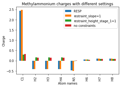
To get an idea for how these changes have affected the output charges, we can organize the methylammonium charges into a Pandas DataFrame and plot them.

[14]:

atom_names = [f"{x}{i}" for i, x in enumerate(methylammonium.qcmol.symbols, 1)]

df = pd.DataFrame({
    "Atom names": atom_names,
    "RESP": normal_charges[1],
    "restraint_slope=1": slope_1[1],
    "restraint_height_stage_1=1": height_1[1],
    "no constraints": no_constraints[1]
})

df.set_index("Atom names", inplace=True)

df.plot(ylabel="Charge", title="Methylammonium charges with different settings", kind="bar");

../_images/examples_04_example_resp_minimal_27_0.png

Using Pandas is quite useful; DataFrames can be saved to CSV files, for example, with df.to_csv(). They can also simply be viewed as a table in a Jupyter notebook.

[15]:

df

[15]:

	RESP	restraint_slope=1	restraint_height_stage_1=1	no constraints
Atom names
C1	2.438582	2.475004	0.292915	0.331088
H2	-0.405468	-0.414351	0.161776	0.150576
H3	-0.405468	-0.414351	0.161776	0.150576
H4	-0.405468	-0.414351	0.161776	0.150576
N5	-0.474650	-0.502243	-0.013021	0.005047
H6	0.054494	0.060254	0.059107	0.035507
H7	0.098988	0.105019	0.087835	0.088315
H8	0.098989	0.105019	0.087835	0.088315