RESP

Background

The electrostatic potential \(V\) is the potential generated by the nuclei and electrons in a molecule. At any point in space \(r\), it is:

\[V(\vec{r}) = \sum_{n=1}^{nuclei} \frac{Z_n}{|\vec{r} - \vec{R}_n|} - \int \frac{\rho(\vec{r’})}{|\vec{r} - \vec{r’}|} d\vec{r}\]

If we generate a grid of points around the molecule and evaluate the potential felt at each grid point, we can set up a system of linear equations to determine the partial charges for the atoms in the molecule that would best fit the potential. Because the grid of points is typically generated at certain radii from each atom, forming a “surface layer” around the molecule, the system of linear equations is commonly called “surface constraints” in the code and throughout the documentation.

The equations represented by the constraint matrix can be solved for the charges of best fit, as first published by Singh and Kollman in 1984 [SK84]. In PsiRESP, this is referred to as the “ESP” method. You can add your own charge constraints; please see the section on charge constraints below.

Commonly, a “restrained fit” is performed to derive the final charges [BCCK93, CCBK95, CCBK93]. This is typically known as “RESP”.

The hyperbolic restraint has the form:

\[\chi_{penalty} = a\sum_{n=1}^{nuclei} ((q_{n}^{2} + b^2)^{1/2} – b)\]

\(a\) defines the asymptotic limits of the penalty, and corresponds to restraint_height_stage_1 and restraint_height_stage_2 for the stage 1 and stage 2 fits, respectively. \(b\) defines the width of the penalty, and corresponds to restraint_slope.

If you only want a one-stage fit, the process stops here. In a two-stage fit, the typical charge model in AMBER and CHARMM force fields, the above is repeated. The difference between the stages is in the charge restraints. In the first stage, all charges are free to vary. In the second stage fit, atoms without an equivalence constraint are fixed (i.e. their charges remain static from stage 1). However, atoms within an equivalence constraint are free to vary. In more technical detail, this is the process for each stage:

All charge equivalence constraints are ignored, and the charges of all atoms are free to vary. This includes the hydrogens around sp3 carbons, which we would expect to be symmetric or equivalent.

The charge equivalence constraints are added back in the second stage. For all atoms that are not involved in an equivalence constraint, their charges are fixed to the stage 1 charges. Now the constraint matrix is only solved to calculate the charges of the equivalent atoms.

Note

sp3 carbons where the attached hydrogens are involved in a constraint, are also not given a fixed charge in stage 2 fits, but left free to vary.

Charge constraints

You can add your own charge constraints to the “surface constraints”. These charge constraints can control what charge a group of atoms should sum to (ChargeSumConstraint); this is very useful for example, for making sure that extraneous caps on an amino acid sum to 0. That way the amino acid retains an integer charge in a protein.

Alternatively, you can control whether an atom should have an equivalent charge to another atom (ChargeEquivalenceConstraint). This is useful for enforcing symmetry. The symmetric_methyls and symmetric_methylenes options in psiresp.charge.ChargeConstraintOptions use ChargeEquivalenceConstraint on the hydrogens around an sp3 carbon.

Please see Charge constraints for more information.

Conformational dependence

RESP methods are highly conformation-dependent; it is highly likely that you derive different charges for the same molecule if you use two different conformers. Even the orientation of the molecule can affect the resulting charges. For that reason, it is highly recommended to use multiple conformers and orientations for each molecule.

While users can provide their own, PsiRESP also includes methods for automatic conformer and orientation generation. In particular, the conformers selected for use in calculating charges use the Electrostatically Least-interacting Functional group (ELF) technique, which is used in AM1BCC ELF10.

Please see Conformers for details on the implementation.

Penalty coefficients

The hyperbolic restraint used in a restrained fit is controlled by two parameters: restraint_height (in a two-stage fit, restraint_height_stage_1 and restraint_height_stage_2 for the first and second stages respectively) and restraint_slope. Below is an explanation of how these parameters control the penalty applied to the matrix of linear equations to be solved.

The way to conceptually understand the purpose of the restraint is to “add noise” to the fit and pull the magnitudes of the resulting charges towards 0. When the charges are fitted to the electrostatic potential, they are done so following the classic equation

\[A\vec{x} = \vec{b}\]

Here, \(A\) has no relation to \(a\) in the hyperbolic restraint. Instead, the inverse distances from each atom to each grid point are summed, and then the atom-to-atom Cartesian product of these form the elements of \(A\). These products are followed by the atoms involved in any charge constraints.

Similarly, \(\vec{b}\) has no relation to \(b\) in the hyperbolic restraint; instead, it is the vector of the summed electrostatic potential felt at each grid point, multiplied by the inverse distance to each atom. (If using charge constraints, \(\vec{b}\) also includes the values of the charge constraints).

Without a restraint, we simply solve for \(x\), i.e., the charges. A row of \(A_{i}\) represents the degree of interaction between atom \(i\) with every other atom in the molecule, which is solved for the summed, distance-weighted electrostatic potential \(\vec{b}_{i}\).

However, we can add a penalty to minimize fluctuation in charges. The restraint is only added to the diagonal elements in \(A\), or the self-interacting terms \(A_{i, i}\). The penalty term updates iteratively depending on the charge \(x_{i}\), until the calculated charges converge within a user-specified threshold.

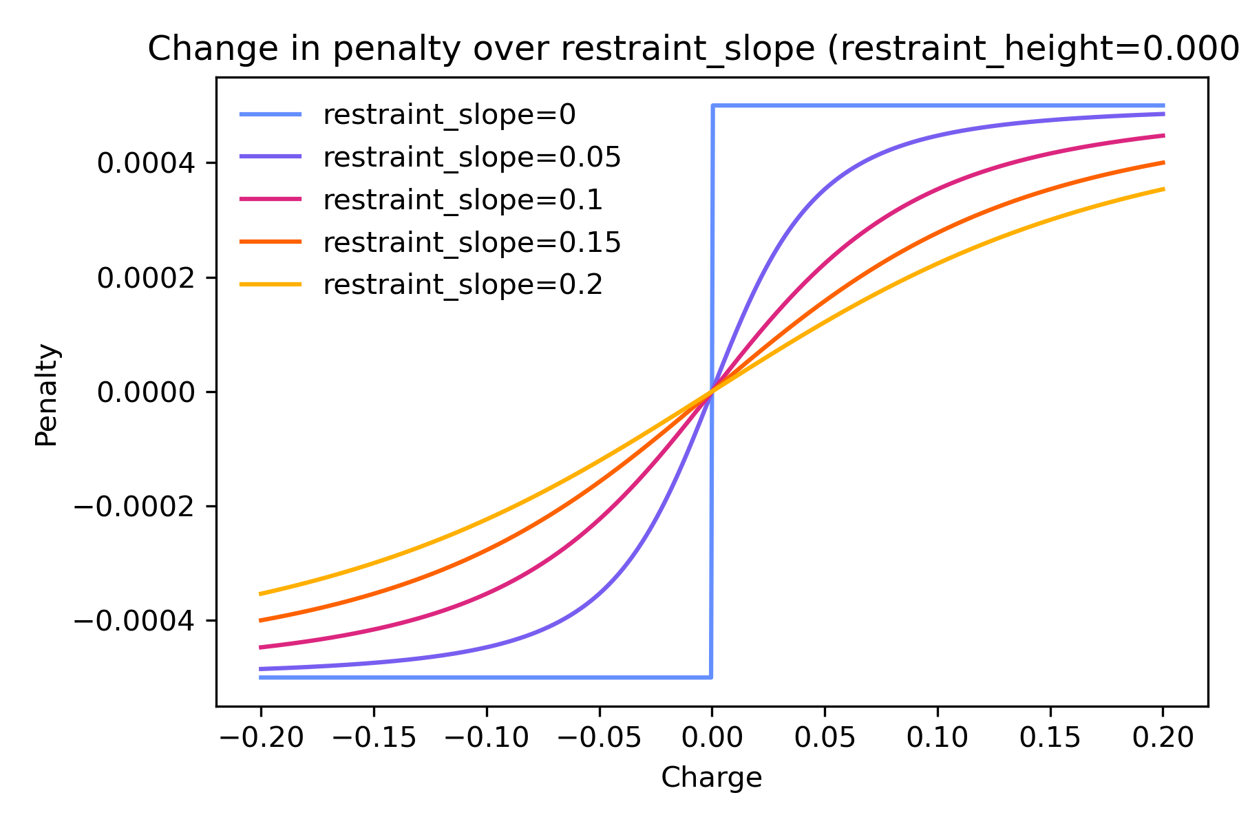
The graphs below illustrate how the penalty added to each term changes with different restraint_height and restraint_slope. restraint_height controls the height of the curve, or the maximum penalty possible no matter how great the charge.

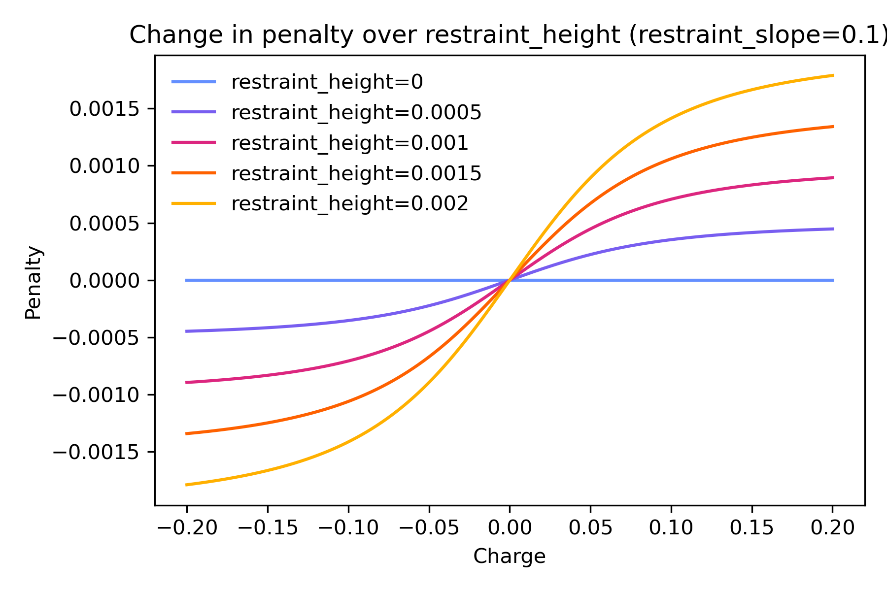
restraint_slope controls the steepness of the curve, or how slowly the penalty changes with the magnitude of charge.

Pre-configured classes

The table below gives a broad overview of the pre-configured classes.

Overview of pre-configured RESP classes
Class	Description	Reference
`psiresp.configs.TwoStageRESP`	A 2-stage restrained fit in the gas phase at hf/6-31g*	Bayly et al. [BCCK93], Cornell et al. [CCBK93], Cieplak et al. [CCBK95]
`psiresp.configs.OneStageRESP`	A 1-stage restrained fit in the gas phase at hf/6-31g*
`psiresp.configs.ESP`	A 1-stage unrestrained fit in the gas phase at hf/6-31g*	Singh and Kollman [SK84]
`psiresp.configs.WeinerESP`	A 1-stage unrestrained fit in the gas phase at hf/sto-3g
`psiresp.configs.ATBRESP`	A 2-stage restrained fit in implicit water at b3lyp/6-31g*	Malde et al. [MZB+11]
`psiresp.configs.RESP2`	A 2-stage restrained fit at pw6b95/aug-cc-pV(D+d)Z, in both vacuum and implicit water. Charges are interpolated between the two phases.	Schauperl et al. [SNJ+20]